Deep Learning

Note: the following notes are based on Stanford Univeristy CS231n: Convolutional Neural Networks for Visual Recognition. The UNSW version of this course lacks in-depth contents and is not as comprehensive as the Stanford version.

Lecture 1

Linear Classifiers

Linear Classifier: y = Wx + b
2-Layer Neural Network: y = W2 * max(0, W1x + b1) + b2

Back propagation

Back propagation is the process of updating the weights of the neural network. The weights of the neural network are updated using the gradient of the loss function with respect to the weights. The gradient of the loss function is calculated using the chain rule. The chain rule is a rule that allows us to calculate the gradient of a function with respect to its inputs.

Neural Networks

A neural network is a series of layers. Each layer is a linear classifier followed by a non-linear activation function. The activation function is a non-linear function that is applied to the output of the linear classifier. This allows the neural network to learn non-linear functions.

Convolutional Layer

We can turn a 32x32x3 image into a huge vector of 3072 elements. This is called the input layer. The output layer is the classification layer. This model could work, but it is not very efficient. We can use a neural network by stacking multiple linear classifiers together. The output of the first linear classifier is the input of the second linear classifier. The output of the second linear classifier is the input of the third linear classifier, and so on. A fully connected neural network is a neural network where each neuron in a layer is connected to every neuron in the next layer.

Fully Connected Layer

As shown above, the filter size always goes full depth, meaning if the input image has three channels, the filter size will also have three channels. The result of taking a dot product between the filter and a small region of the input image is a single number. In essence, it is called convolutional layer because the filter is convolved with the input image. With signal processing, convolution is a mathematical operation that takes two functions and produces a third function. In the context of neural networks, the two functions are the input image and the filter, and the third function is the output of the convolutional layer.

Convolutional Layer

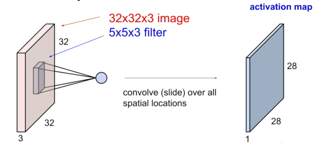
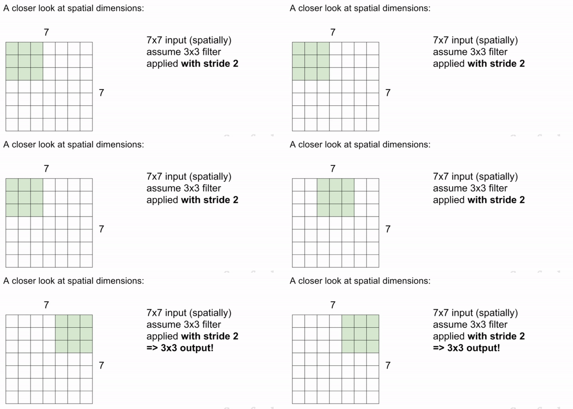
We have the options to slide pixel by pixel, or multiple pixels at a time. The stride is the number of pixels that the filter is moved across the input image. The most common stride values are 1, 2, and 3 (see next section). Also, we can stack as many filters as we want to get a stacked activation map. To use these convolutional layers, we need to use a non-linear activation function. The most common activation functions are: ReLU (Other functions are introduced in the next section).

six_layers

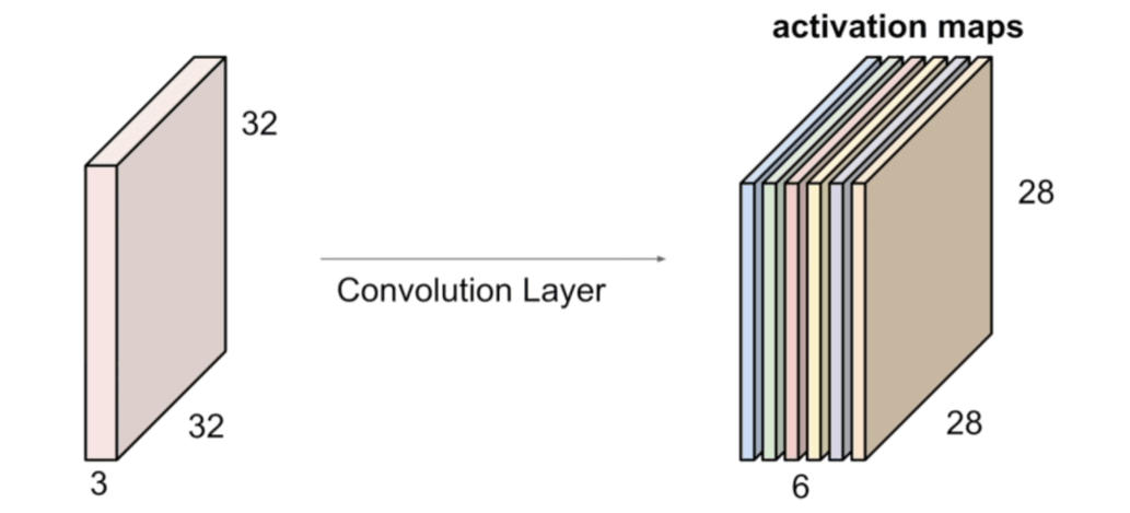
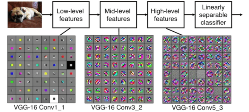
We can visualize this in a VGG16 architecture. The VGG16 architecture is a convolutional neural network that has 16 layers. The VGG16 architecture is composed of 13 convolutional layers and 3 fully connected layers.

VGG16

Filter Size

The filter size is the size of the filter that is applied to the input image. The filter size is usually a square matrix with odd dimensions. The most common filter sizes are 3x3, 5x5, and 7x7.

Filter

Stride

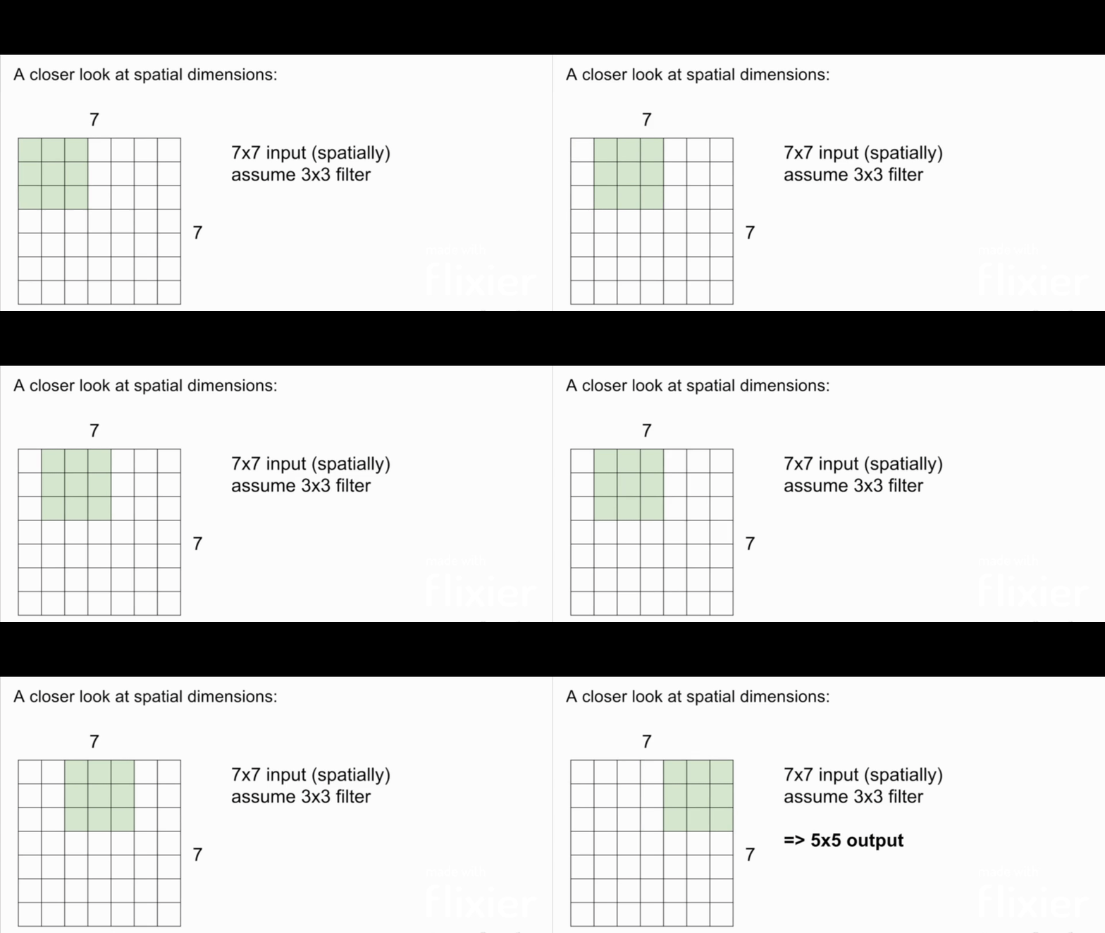
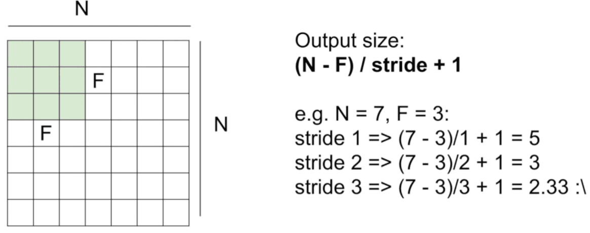
Stride is the number of pixels that the filter is moved across the input image. The most common stride values are 1, 2, and 3. Note: in this case, if we use stride 3 in the below image, it doesn't work because asymmetry is introduced.

Stride

Padding

Padding is the process of adding zeros to the input image. Padding is used to ensure that the output image has the same dimensions as the input image. The most common padding methods are:

Valid padding: no padding
Same padding: padding is added to the input image so that the output image has the same dimensions as the input image. In practice: it is common to zero pad the border of the input image so that the output image has the same dimensions as the input image. This is called same padding.

Padding

Example Questions

Question 1

Input Volume: 32x32x3 Filter Size: 5x5x3 Number of Filters: 10 Stride: 1 Padding: 2

What is the output volume?

Answer: Output Volume: 32x32x10

Question 2 Input Volume: 32x32x3 Filter Size: 5x5x3 Number of Filters: 10 Stride: 1 Padding: 2

Number of parameter in this layer?

Answer: Number of parameters: 5x5x3x10 + 10 = 760 (5x5x3 is the filter size, 10 is the number of filters, or bias term)

Common Settings K = (powers of 2) 32, 64, 128, 256, 512, 1024 - F = 3, S = 1, P = 1 - F = 5, S = 1, P = 2 - F = 5, S = 2, P = whatever fits - F = 3, S = 2, P = 0

Pooling

Pooling is the process of reducing the dimensions of the input image. Pooling is used to reduce the number of parameters in the neural network. The most common pooling methods are:

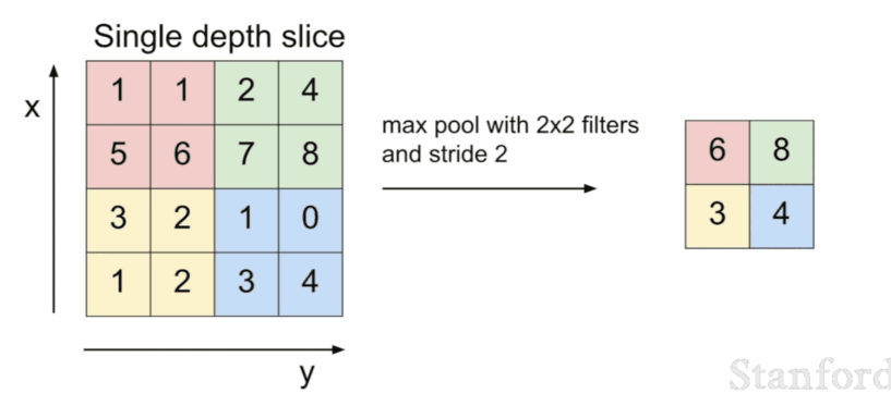
Max pooling: the maximum value in the filter is selected
Average pooling: the average value in the filter is selected

For example, we have a 2x2 filter and we apply max pooling to the input image. The output image will have half the dimensions of the input image.

Pooling

In the end, we want to have a fully connected layer which connects to the entire input volume, as in original neural networks.

Dilation

Dilation is the process of adding zeros to the input image. Dilation is used to increase the receptive field of the filter. The most common dilation values are 1, 2, and 3.

Activation Function

The activation function is a non-linear function that is applied to the output of the linear classifier. The activation function is what allows the neural network to learn non-linear functions. The most common activation functions are:

Sigmoid: $f(x) = \frac{1}{1 + e^{-x}}$
Tanh : $f(x) = \frac{e^x - e^{-x}}{e^x + e^{-x}}$
ReLU: $f(x) = max(0, x)$ mostly used
Leaky ReLU: $f(x) = max(0.01x, x)$
Maxout: $f(x) = max(w_1^Tx + b_1, w_2^Tx + b_2)$

Lecture 2 HyperParameters-Tuning and Optimization

Preprocessing the data

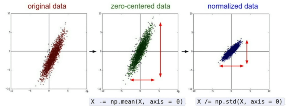
zero-centering: subtract the mean of the data from the data, we need to apply this to both the training and test phase. zero_center

subtract the mean image (e.g. AlexNet)
subtract per channel mean (e.g. VGGNet)

normalization: divide the data by the standard deviation of the data, we don't need this for this course

PCA: Principal Component Analysis, we don't need this for this course

whitening: zero-centering and normalization, we don't need this for this course

Weight Initialization

Xavier initialization [Glorot et al. 2010]

W = np.random.randn(fan_in, fan_out) / np.sqrt(fan_in)

He et al., 2015, use this for our project

W = np.random.randn(fan_in, fan_out) / np.sqrt(fan_in / 2)

Batch Normalization

[loffe and Szegedy, 2015]

Batch normalization is a technique that is used to normalize the input to a neural network. Batch normalization is used to speed up the training

Steps

Data Preprocessing
Choose the architecture

Double check the loss function

model = your model(input_size, hidden_size, num_classes)
loss, grad = model.loss(X_train, model, y_train, 0) # disable regularization
loss, grad = model.loss(X_train, model, y_train, 1e3) # crank up regularization, if loss goes up, good
print(loss)

Adjust learning rate, 1e-3, 1e-4, 1e-5, 1e-6 etc. Run coarse search for 5 epochs, then fine search for 20 epochs.
Hyperparameter search using random search [Bergstra and Bengio, 2012]

Week5 Week8