Image Processing

Lecture 1 Image Processing Part I

Neighbourhood Operations

Spatial Filtering

Use the gray values in a small neighbourhood of a pixel in the input images to produce a new gray value for that pixel in the output image. Depending on the weights applied to pixel values, the output image can be blurred, sharpened, or otherwise modified.

Below is a code snippet to apply a filter to an image.

import cv2
import numpy as np
 
def apply_filter(image, kernel):
    return cv2.filter2D(image, -1, kernel)
 
image = cv2.imread('image.jpg', cv2.IMREAD_GRAYSCALE)
kernel = np.array([[0, -1, 0], [-1, 5, -1], [0, -1, 0]])
filtered_image = apply_filter(image, kernel)
 
cv2.imshow('Original Image', image)
cv2.imshow('Filtered Image', filtered_image)
cv2.waitKey(0)
cv2.destroyAllWindows()

Neighbourhood of a pixel is defined by a window of size n x n where n is an odd number. The pixel is at the center of the window. Typical kernel sizes are 3 x 3, 5 x 5, 7 x 7, etc. but can be larger and have different shapes.

Convolution

The output image o(x,y) is computed by discrete convolution the input image i(x,y) with a kernel h(x,y) as follows:

$o(x,y) = \sum*{i=-n}^{n} \sum*{j=-m}^{m} f(x-i, y-j) h(i,j)$

where a and b are half the dimensions of the kernel. The kernel is flipped both horizontally and vertically before the convolution.

where the sum is over all s and t for which the kernel is defined.

For example, consider a 3x3 kernel:

$h = \begin{bmatrix} 1 & 2 & 3 \\ 4 & 5 & 6 \\ 7 & 8 & 9 \end{bmatrix}$

The convolution operation is:

$o(x,y) = f(x-1, y-1) \times 1 + f(x-1, y) \times 2 + f(x-1, y+1) \times 3 + f(x, y-1) \times 4 + f(x, y) \times 5 + f(x, y+1) \times 6 + f(x+1, y-1) \times 7 + f(x+1, y) \times 8 + f(x+1, y+1) \times 9$

The convolution operation is performed for each pixel in the image. The output image is the result of the convolution operation. Here x is the row and y is the column of the image.

Border Problem

This boundary pixels are not included in the convolution operation. This is called the border problem. The output image will be smaller than the input image.

There are several ways to handle the border problem:

1. Padding: Add a border of zeros around the image, if you have a 3x3 kernel size, the padding of the image will be 1 pixel, and if you have a 5x5, you will need to pad with 2 pixels
2. Clamping: Repeat all the pixels at the border. This has better border behaviour but arbitary
3. Wrapping: Copy pixel values from the opposite side of the image. Implicitly used in fast fourier transformation
4. Mirroring: Reflect pixel values across borders, smooth, symmetric, periodic, no boundary artifacts

Linear shift-invariant operations

• Linear: only addition and multiplication are used in the operation
• shift-invariant: if f(x,y) generates an output g(x, y), then the shifted input $f(x + \Delta x, y + \Delta y)$ yileds the shifted output $g(x + \Delta x, y + \Delta y)$. In other words, the operation does not discriminate between spatial operations

Filtering Methods

Uniform Filter

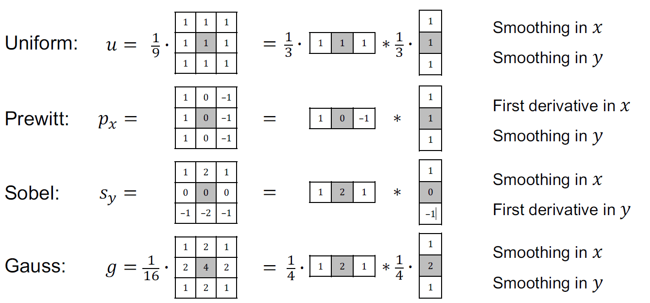
Simplest smoothing filter: mean pixel value filter. It is often used in image processing to reduce noise, but it also blurrs the image.

to calculate the mean pixel value, you need to sum all the pixel values and divide by the number of pixels

$g(x, y) = \frac{1}{|N|} \sum*{i=-1}^{N} \sum*{j=-1}^{N} f(x+i, y+j)$

def uniform_filter(image, kernel_size):
    kernel = np.ones((kernel_size, kernel_size), np.float32) / (kernel_size * kernel_size)
    return cv2.filter2D(image, -1, kernel)

Gaussian Filter

$g(x, y) = \frac{1}{2\pi \sigma^2} \exp(-\frac{x^2 + y^2}{2\sigma^2})$

The Gaussian filter gives more weight to the central pixel and less weight to the pixels further away from the center. It is separable, which means that it can be applied in two steps, first in the x direction and then in the y direction. It is also circular symmetric, which means that it is the same in all directions. The sigma parameter controls the amount of smoothing. The larger the sigma, the more smoothing.

def gaussian_filter(image, kernel_size, sigma):
    return cv2.GaussianBlur(image, (kernel_size, kernel_size), sigma)

The sigma parameter controls the amount of smoothing. The larger the sigma, the more smoothing. Some common values for sigma are 0.5, 1, 2, 3, 4, 5, etc.

Median Filter

For median filter, instead of taking the mean of the pixel values, you take the median.

• The pixels with distinct intensity values are replaced by the median value of the pixels in the neighbourhood.
• It is not a convolution filter, but a non-linear filter.
• It is used to remove salt and pepper noise.
• Neighbourhood is typically of size 3x3 or 5x5.
• This also eliminates pixel clusters with area < $\frac{n^2}{2}$

We can use opencv to do media Filtering

def median_filter(image, kernel_size):
    return cv2.medianBlur(image, kernel_size)

You have two variations of median filter, if you take the minimum and maximum insteawd of the median, you get the min filter and max filter respectively. Gaussian filter is better when we need to retain small details in the image, while median filter is better when we need to remove salt and pepper noise.

Image Enhancement

Unsharp Masking

Smoothing kernels can also be used to sharpen images using a process called unsharp masking. Since blurring the image reduces high frequencies, adding some of the difference between the original and the blurred image makes it sharper.

$g(x, y) = f(x, y) + k(f(x, y) - f'(x, y))$

where f(x, y) is the original image, f'(x, y) is the blurred image, and k is a scaling factor. In the lecture example, the input cat minus the Gaussian cat gives the high frequency components of the image. Adding this to the original image gives a sharper image.

Pooling

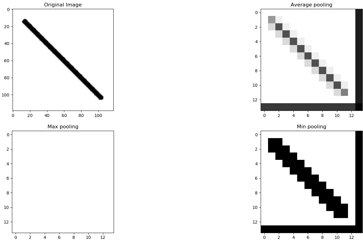
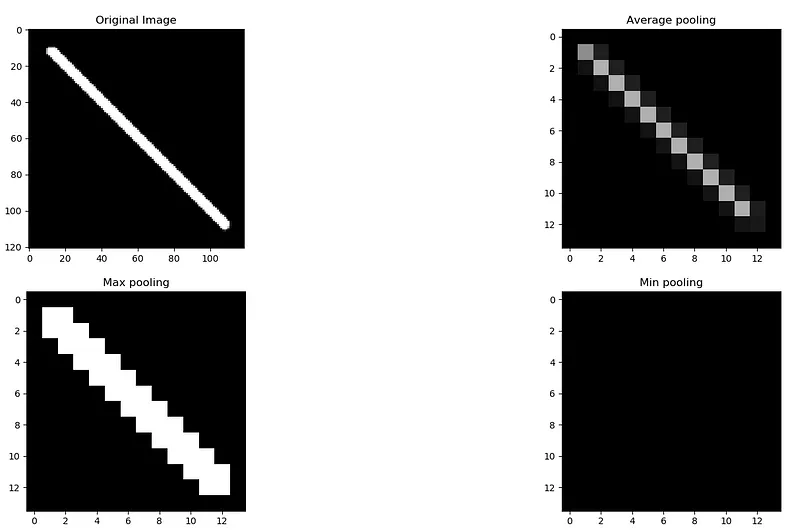
Pooling is nothing other than down sampling of an image. The most common pooling layer filter is of size 2x2, which discards three forth of the activations.

• Combines filtering and downsampling in one step
• Examples include max, min, median, average pooling
• Makes the image smaller and reduces computations
• Popular in deep convolutional neural networks

The Max Pooling layer summarizes the features in a region represented by the maximum value in that region. Max Pooling is more suitable for images with a dark background as it will select brighter pixels in a region of the input image.

The Min Pooling layer summarizes the features in a region represented by the minimum value in that region. Contrary to Max Pooling in CNN, this type is mainly used for images with a light background to focus on darker pixels.

The average pooling summarizes the features in a region represented by the average value of that region. With average pooling, the harsh edges of a picture are smoothened, and this type of pooling layer can used when harsh edges can be ignored.

def max_pooling(image, kernel_size):
    return cv2.dilate(image, np.ones((kernel_size, kernel_size), np.uint8))
 
def min_pooling(image, kernel_size):
    return cv2.erode(image, np.ones((kernel_size, kernel_size), np.uint8))
 
def average_pooling(image, kernel_size):
    return cv2.blur(image, (kernel_size, kernel_size))

Edge detection

Derivative filters

First order: mainly used in edge detection

• Gradient domain filtering
• Spatial derivatives respond to intensity changes
• In digital images they are approximated using finite differences
• Different possible ways to take finite differences

Sobel filter

$S_x = \begin{bmatrix} 1 & 0 & -1 \\ 2 & 0 & -2 \\ 1 & 0 & -1 \end{bmatrix}$

$S_y = \begin{bmatrix} 1 & 2 & 1 \\ 0 & 0 & 0 \\ -1 & -2 & -1 \end{bmatrix}$

Prewitt filter

$P_x = \begin{bmatrix} 1 & 0 & -1 \\ 1 & 0 & -1 \\ 1 & 0 & -1 \end{bmatrix}$

$P_y = \begin{bmatrix} 1 & 1 & 1 \\ 0 & 0 & 0 \\ -1 & -1 & -1 \end{bmatrix}$

Pay attention to the signs of the filters, if the center pixel is negative, the filter is second order derivative, if the center pixel is positive, the filter is first order derivative or smoothing.

def sobel_filter(image):
    sobelx = cv2.Sobel(image, cv2.CV_64F, 1, 0, ksize=5)
    sobely = cv2.Sobel(image, cv2.CV_64F, 0, 1, ksize=5)
    return sobelx, sobely
 
def prewitt_filter(image):
    kernelx = np.array([[1, 0, -1], [1, 0, -1], [1, 0, -1]])
    kernely = np.array([[1, 1, 1], [0, 0, 0], [-1, -1, -1]])
    prewittx = cv2.filter2D(image, -1, kernelx)
    prewitty = cv2.filter2D(image, -1, kernely)
    return prewittx, prewitty

Laplacian filter

The Laplacian filter is a second order derivative filter. It is used to detect edges and fine details in an image. It is also used to detect zero-crossings (A zero-crossing is a point where the sign of a mathematical function changes (e.g. from positive to negative), represented by an intercept of the axis in the graph of the function) in an image. Compared to Sobel and Prewitt filters:

• the Laplacian filter is more sensitive to noise
• Sobel and Prewitt filters measure the gradient magnitude, while the Laplacian filter measures the change in gradient magnitude
• Sobel and Prewitt filters work on the first derivative of the image and produce results highlighting edges where there is a rapid change in intensity.

Sharpending using Laplacean

$g(x, y) = f(x, y) + k \nabla^2 f(x, y)$

where $\nabla^2 f(x, y) = \frac{\partial^2 f(x, y)}{\partial x^2} + \frac{\partial^2 f(x, y)}{\partial y^2}$

The reason why the Laplacian filter is used for sharpening is that it highlights the edges in the image. The edges are the areas where the intensity changes rapidly. By adding the Laplacian of the image to the original image, the edges are enhanced.

# implementation of laplacian filter sharpening image
def laplacian_filter(image):
    laplacian = cv2.Laplacian(image, cv2.CV_64F)
    return laplacian
 
# implementation from scratch
def laplacian_filter(image):
    kernel = np.array([[0, 1, 0], [1, -4, 1], [0, 1, 0]])
    return cv2.filter2D(image, -1, kernel)

Example exam question What is the effect of the 2D convolution kernalshown on the right when applied to an image? $k = \begin{bmatrix} 0 & 1 & 0 \\ 1 & -4 & 1 \\ 0 & 1 & 0 \end{bmatrix}$

• A. It approximates the sum of first-order derivatives in 𝑥 and 𝑦.
• B. It approximates the sum of second-order derivatives in 𝑥 and 𝑦.
• C. It approximates the product of first-order derivatives in 𝑥 and 𝑦.
• D. It approximates the product of second-order derivatives in 𝑥 and 𝑦.

Lecture 2 Image Processing Part II

Transform Domain Filtering (Fourier Transform)

What is lost when lowering the resolution of an image?

• A. Image quality
• B. Image size
• C. Image details
• D. Image color

The answer is C. Image details. This is down sampling, which is a form of pooling.

Spatial versus frequency domain

• Spatial domain: image is represented as a 2D array of pixel values, we can apply filters directly to the image, the changes are local, meaning that the changes are applied to the pixel values directly
• Frequency domain: image is represented as a sum of sinusoidal functions, we can apply filters to the frequency components of the image, the changes are global, meaning that the changes are applied to the frequency components of the image

Some key points:

• high frequency components correspond to rapidly changing intensities across pixels (often edges and fine details)
• low frequency components correspond to large-scale image structures (often smooth regions)

1D Fourier Transform

Basic idea of Fourier Transform

Let's look at a sinusode function:

$f_1(x) = a_i\sin(w_ix + \phi_i)$

where $a_i$ is the amplitude, $w_i$ is the radial frequency, and $\phi_i$ is the phase.

Add all the sines and cosines together to get the original signal, you can have f = f_0 + f_1 + f_2 + ... + f_n. Note that there is no loss of information during the Fourier Transform.

• f(x) -> Fourier Transform -> F(u)
• F(u) -> Inverse Fourier Transform -> f(x)

Fourier Transform: $F(u) = \int_{-\infty}^{\infty} f(x)e^{-i2\pi wx}dx$

Inverse Fourier Transform: $f(x) = \int_{-\infty}^{\infty} F(u)e^{i2\pi wx}dx$

2D Fourier Transform

Forward Fourier Transform: $F(u, v) = \int_{-\infty}^{\infty} \int_{-\infty}^{\infty} f(x, y)e^{-i2\pi(ux+vy)}dxdy$

Inverse Fourier Transform: $f(x, y) = \int_{-\infty}^{\infty} \int_{-\infty}^{\infty} F(u, v)e^{j2\pi(ux+vy)}dudv$

Discrete Fourier Transform

The Discrete Fourier Transform (DFT) is a sampled version of the Fourier Transform. The DFT is used to transform a digital image into its frequency components.

Forward Discrete Fourier Transform: $ F(u, v) =

Inverse Discrete Fourier Transform: $ f(x, y) =

Filtering procedure

1. Multiply the input image f(x, y) by (-1)^(x+y) to center the transform
2. Compute the transform F(u, v) from image f(x, y) using the 2D DFT
3. Multiply F(u, v) by a centered filter H(u, v) to obtain G(u, v)
4. Compute the inverse 2D DFT of G(u, v) to obtain the spatial result g(x, y)
5. Take the real part of g(x, y)
6. Multiply the result by (-1)^(x+y) to remove the pattern introduced in 1

Low pass filtering

Low pass filter passes low frequency components and blocks high frequency components. It is used to smooth or blur an image.

High pass filtering

High pass filter passes high frequency components and blocks low frequency components.

Notch filtering

Notch filtering is used to remove specific frequencies from an image. It is used to remove periodic noise from an image.

Phase vs Magnitude

The magnitude of the Fourier Transform represents the amount of each frequency component in the image. The phase of the Fourier Transform represents the position of each frequency component in the image. If you only change the magnitude of the Fourier Transform, you will change the intensity of the image. If you only change the phase of the Fourier Transform, you will change the position of the image. Sometimes, phase information is more important than magnitude information. For example, if you only preserve the magnitude of the Fourier Transform, you will get a blurry image, sometimes not even making sense. But if you only preserve the phase of the Fourier Transform, you will get a sharp image, but the intensity will be lost.

Some examples can be found in this YouTube Video (opens in a new tab)

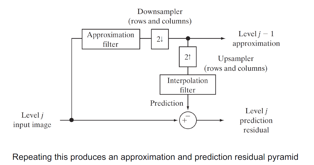
Multiresolution image processing

• Small objects and fine details benefit from high resolution
• Large objects and coarse structures can make do with low resolution
• If both are needed, use multiresolution image processing

Creating image pyramids

1. Compute the Gaussian pyramid (approximation pyramid) of the input image by applying a low pass filter and downsampling

2. Upsample the output of step 1 and apply a low pass filter to get the residual pyramid (detail pyramid)

3. Compute the difference to get residual pyramid: also called laplacian pyramid because it is the difference between the original image and the upsampled image

Example exam question

Which one of the following statements on image filtering is incorrect? A. Median filtering reduces noise in images. B. Low-pass filtering results in blurry images. C. High-pass filtering smooths fine details in images. D. Notch filtering removes specific image frequencies

The answer is C. High-pass filtering enhances edges and fine details in images.