Introduction and Image Formation

Lecture 1 Image Formation

• Lab consultations: Wednesdays 6-7pm in weeks 2-5 (via BB Collab) Software demos and consultations with your assigned tutor (links in Moodle)

  Lab Work (4x) 10% Weeks 2, 3, 4, 5 Weeks 3, 4, 5, 7 Online

• Project consultations: Wednesdays 6-7pm in weeks 6-10 (via BB Collab) All project consultations will be online with your assigned tutor (links in Moodle)

  Group Project 40% Week 5 Week 10 Online

Color Spaces

• RGB:

  • Red, Green, Blue,
  • Additive color model,
  • 3 channels, 8 bits per channel, 24 bits per pixel, 16.7 million colors,
  • Drawback of RGB: channels are strongly correlated, not a efficient way to model

• HSV:

  • Hue, Saturation, Value,
  • cylindrical color model,
  • 3 channels, 8 bits per channel, 24 bits per pixel, 16.7 million colors,
  • Hue: 0-360 degrees, Saturation: 0-100%, Value: 0-100%,
  • Drawback of HSV: confounded channels by the fact that it is not perceptually uniform

• YCbCr:

  • Luminance, Chrominance Blue, Chrominance Red,
  • 3 channels, 8 bits per channel, 24 bits per pixel, 16.7 million colors,
  • Used in JPEG compression, used in television and video compression,

• Lab:

  • Lightness, a, b, a refers to the green-red component, b refers to the blue-yellow component,
  • 3 channels, 8 bits per channel, 24 bits per pixel, 16.7 million colors
  • Any numerical change in Lab space is perceptually uniform, this is what we use in image processing

Example exam question Which one of the following statements about colour spaces is incorrect? A. The R, G, and B channels of the RGB colour space are often correlated. B. The H and the S channel of the HSV colour space are confounded. C. The Y channel of the YCbCr colour space represents the brightness. D. The a* channel of the Lab* colour space is the green-blue component.

The answer is D, the a* channel of the Lab* colour space is the red-green component.

Face Recognition

Spatial resolution is the number of pixels in an image, the higher the resolution the more detail in the image. For face recognition, we need to have a high spatial resolution to capture the details of the face. Usually we need a resolution of 64x64 pixels.

Lecture 2 Image Processing

What is image processing

• image processing = image in -> image out
• image analysis = image in -> features out
• computer vision = image in -> interpretation out

Categories of image processing

Spatial domain: pixel-based operations

• point operations: operate on individual pixels, such as contrast stretching, thresholding, inversion, log/power transformations
  • T operates on a single pixel
  • T: $R -> R,\ g(x, y) = T(f(x, y))$
• neighbourhood operations: operate on a group of pixels
  • T operates on a group of pixels
  • T: $R^n -> R,\ g(x, y) = T(f(x, y), f(x+1, y), f(x-1, y),...)$

Contrast stretching

• Puts values below L in the input to the minimum (black) in the output
• Puts values above H in the input to the maximum (white) in the output
• Linearly scales values between L and H in the input to between the minimum and maximum in the output

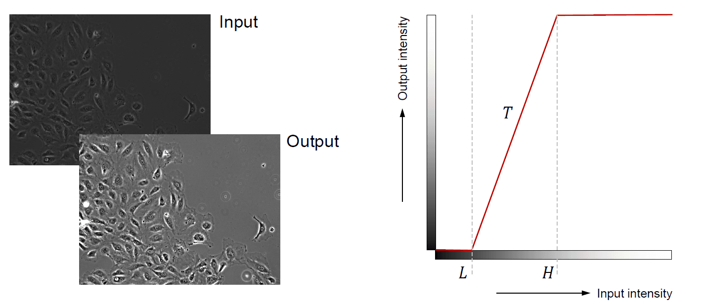
Intensity thresholding

• Binary thresholding: $g(x, y) = 1$ if $f(x, y) > T$, $g(x, y) = 0$ otherwise
• If you reduce the threshold, you will get more white pixels
• If you increase the threshold, you will get more black pixels

Automatic intensity thresholding

Otsu's method

Exhaustively searches for the threshold that minimizes the intra-class variance: $\sigma^2_w = p_0\sigma^2_0 + p_1\sigma^2_1$ . Equivalently, maximizes the inter-class variance: $\sigma^2_b = p_0p_1(\mu_0 - \mu_1)^2$. Here p_0 is the probability of class 0, p_1 is the probability of class 1, $\sigma^2_0$ and $\sigma^2_1$ are the variances of the two classes, and $\mu_0$ and $\mu_1$ are the means of the two classes.

IsoData method

• Start with an initial threshold value
• Compute the mean of the pixels below the threshold and the mean of the pixels above the threshold
• Update the threshold to the average of the two means t = (mean1 + mean2) / 2
• Repeat until the threshold converges

Multilevel thresholding: Apply thresholding multiple times to segment an image into multiple regions

Invensity Inversion

• Apply thresholding to segment the image into two regions
• Invert the intensity values of one of the regions

Log/Power transformation

• Logarithmic transformation: $s = c \log(1 + r)$, they are non-linear mapping, so we can map a relatively narrow range of input values to a wider range of output values
• Power-law (gamma) transformation: $s = c r^{\gamma}$, they map a relatively wide range of input values to a narrow range of output values

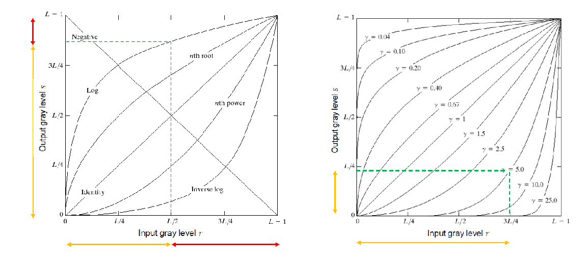
Piecewise linear transformations

• Piecewise linear transformation: $s = T(r)$, where T is a piecewise linear function
• complementary to other transformations, such as contrast stretching

Grey-level slicing

• High value for all grey levels in a range of interest and low values for all others
• Useful for highlighting a specific range of intensities

Histogram of pixel values

• The histogram can be used to determine the contrast of an image, brightness of an image, and the distribution of pixel values in an image

Histogram based thresholding

• Find the histogram peak ($r_p, h_p$) and the highest greay level point ($r_{max}, h_{max}$)
• Construct a line between the peak and the highest grey level point
• Find the gray level r for which the distance between the line and the histogram is maximized

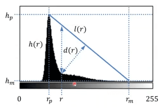
Histogram equalization

• Enhances contrast for intensity values near histogram maxima and decreases contrast near histogram minima
• The cumulative distribution function (CDF) is used to map the input intensity values to the output intensity values
• p_s(s) = p_r(r)dr/ds, where p_s(s) is the probability density function of the output intensity values, p_r(r) is the probability density function of the input intensity values, and dr/ds is the derivative of the CDF

$p_s(s) = \frac{p_r(r)}{(L-1)p_r(r)} = \frac{1}{L - 1}$

• The discrete form of the CDF is used to map the input intensity values to the output intensity values
• p_r(r_k) = n_k / N, where n_k is the number of pixels with intensity r_k, and N is the total number of pixels

$s_k = (L-1) \sum_{j=0}^{k} p_r(r_j) = \frac{(L-1)}{M \times N} \sum_{j=0}^{k} n_j$

The difference between cumulative and discrete CDF is that the cumulative CDF is the integral of the probability density function, while the discrete CDF is the sum of the probability density function

We also have constrained historgam equalization, where we can specify the desired histogram to slow down the contrast enhancement (gradient growth rate) in some regions of the image

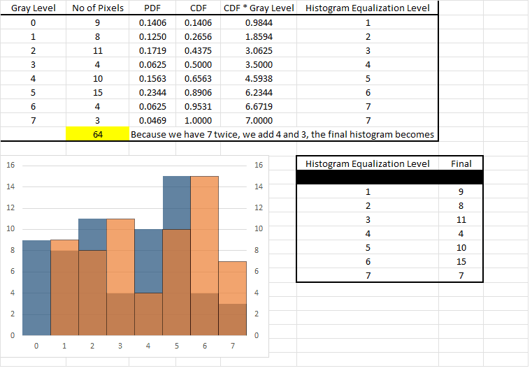
We can see that the blue histogram is smoothed out, and the orange histogram is the equalized histogram

Histogram matching

• Match the histogram of an input image to the histogram of a reference image

Assume that r and s are continuous and $p_z(z)$ is the target distribution for the output image. So we can apply the following transformation:

$s = T(r) = (L-1)\int_{0}^{r} p_r(\zeta)d\zeta$

Now we can define another function G(s) as:

$G(z) = (L-1)\int_{0}^{z} p_z(\zeta)d\zeta = s$

Therefore:

$z = G^{-1}(s) = G^{-1}[T(r)]$

For discrete image values we can write:

$s_k = T(r_k) = (L-1)\sum_{j=0}^{k} p_r(r_j) = \frac{(L-1)}{M \times N} \sum_{j=0}^{k} n_j$

And $G(z_q) = (L - 1)\sum_{i=0}^{q} p_z(z_i)$

Therefore we can write:

$z_q = G^{-1}(s_k)$

The difference between histogram equalization and histogram matching is that histogram equalization enhances the contrast of an image, while histogram matching matches the histogram of an input image to the histogram of a reference image

Example:

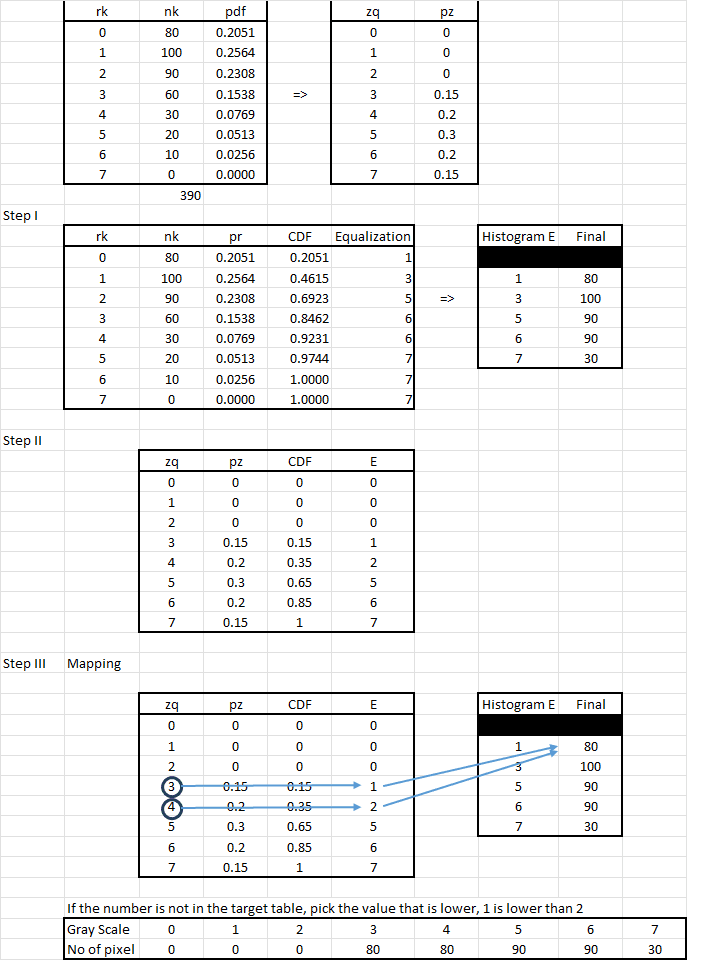
Suppose that a 3-bit image (L = 8) of size 64x64 pixels (MN=4096) has the following intensity distribution shown in the following table (on the left). Get the histogram transformation function and make the output image match the specified histogram, listed in the table on the right.

Arithmetic operations on images:

• Addition: $g(x, y) = f_1(x, y) + f_2(x, y)$
• Subtraction: $g(x, y) = f_1(x, y) - f_2(x, y)$
• Multiplication: $g(x, y) = f_1(x, y) \times f_2(x, y)$
• Division: $g(x, y) = f_1(x, y) / f_2(x, y)$
• Logical operations: AND, OR, XOR, NOT Applications: image blending, image subtraction, image division, image masking

Averaging

Application: reduce noise in images

Assume the true noise free image is $g(x, y)$ and the noisy image is $f_i(x, y) = g_i(x, y) + n_i(x, y)$ for i = 1...n, where n(x, y) is the zero mean independent and identically distributed noise. We can write the average of the noisy images as:

$E[f_i(x, y)] = g(x, y)$ and VAR[$n_i(x, y)$] = $\sigma^2(x, y) \rightarrow$ $\overline f(x, y) = \frac{1}{n} \sum_{i=1}^{n} f_i(x, y) = g(x, y) + \frac{1}{n} \sum_{i=1}^{n} n_i(x, y)$

Question: What is the variance and standard deviation of the average image?

$VAR[\overline f(x, y)] = \frac{1}{n^2} \sum_{i=1}^{n} VAR[n_i(x, y)] = \frac{1}{n^2} \sum_{i=1}^{n} \sigma^2(x, y) = \frac{1}{n} \sigma^2(x, y)$

The standard deviation of the average image is $\frac{\sigma(x, y)}{\sqrt{n}}$

Example exam question

Which one of the following statements about intensity transformations is correct?

• A. Contrast stretching linearly maps intensities between two values to the full output range
• B. Logarithmic transformations maps a narrow range of high intensities to a wider range of output values
• C. Power transformation can map intensities similar to log and inverse log transformations
• D. Piecewise linear transformations are complementary to other transformations

Explanation: B is incorrect because logarithmic transformation maps a narrow range of low-intensity input values to a wide range of output values. C is incorrect because they do not map intensities in a similar manner to log and inverse log transformations. D is incorrect because they are not necessarily complementary but are instead an alternative approach to intensity transformation.